×
![]()
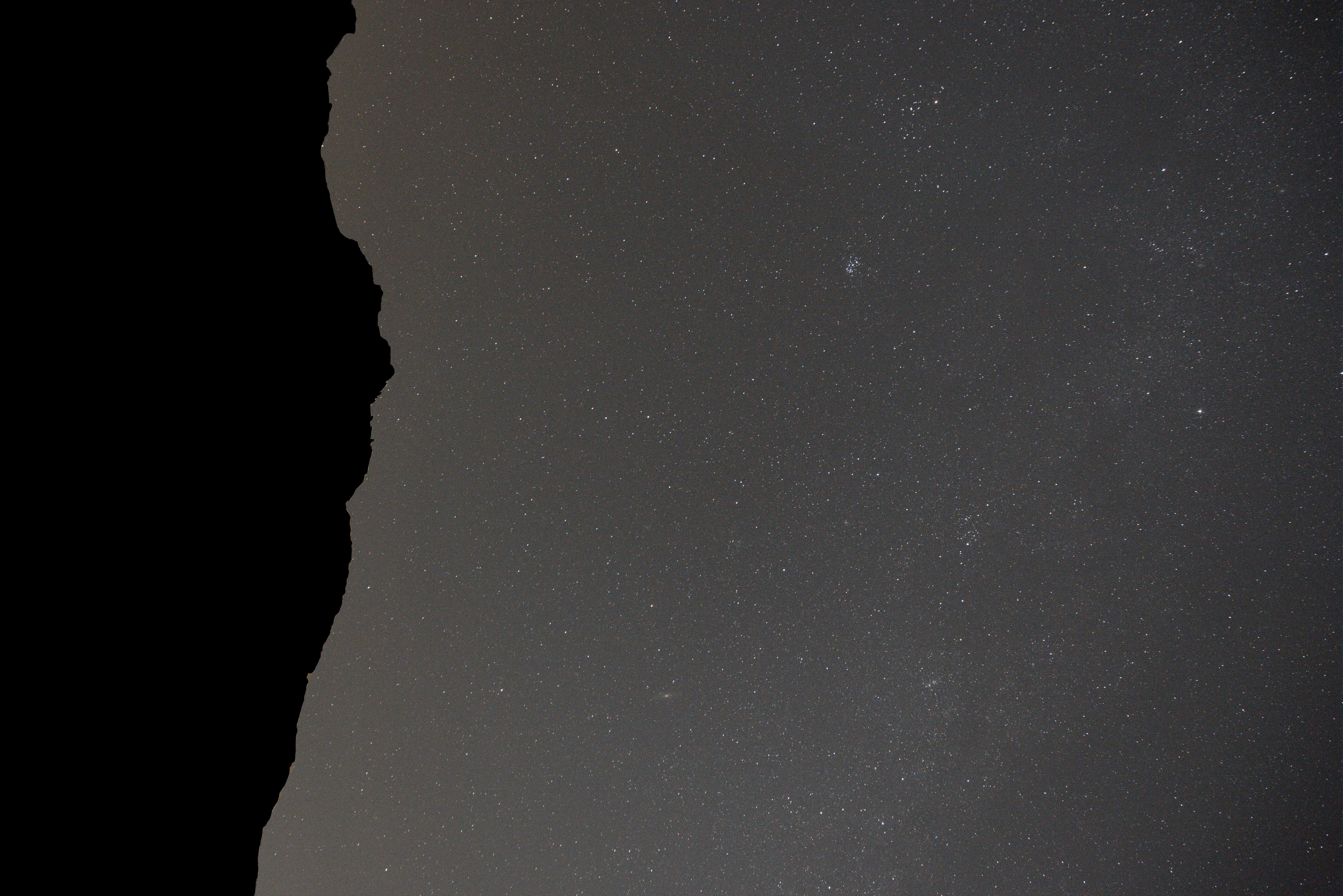
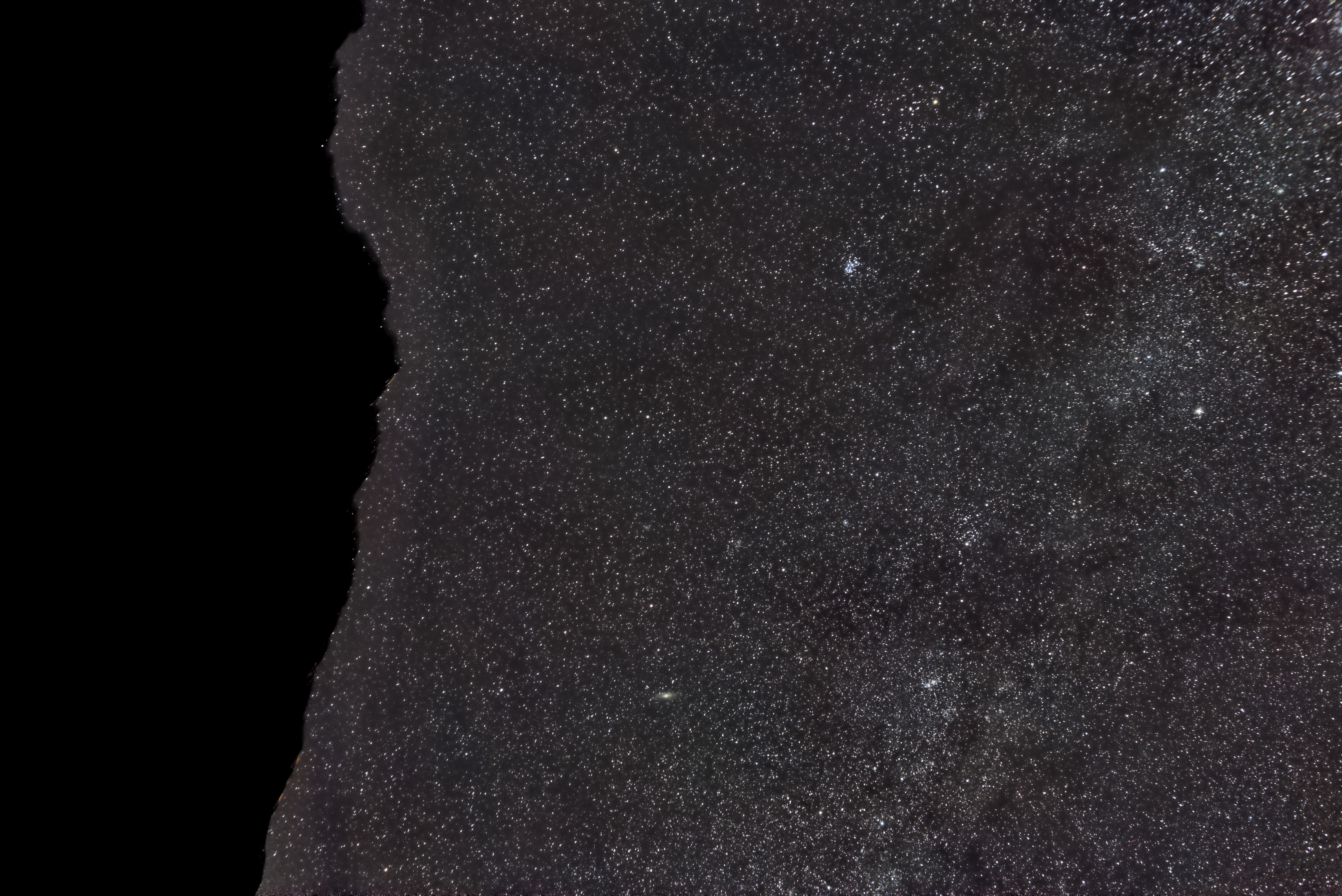
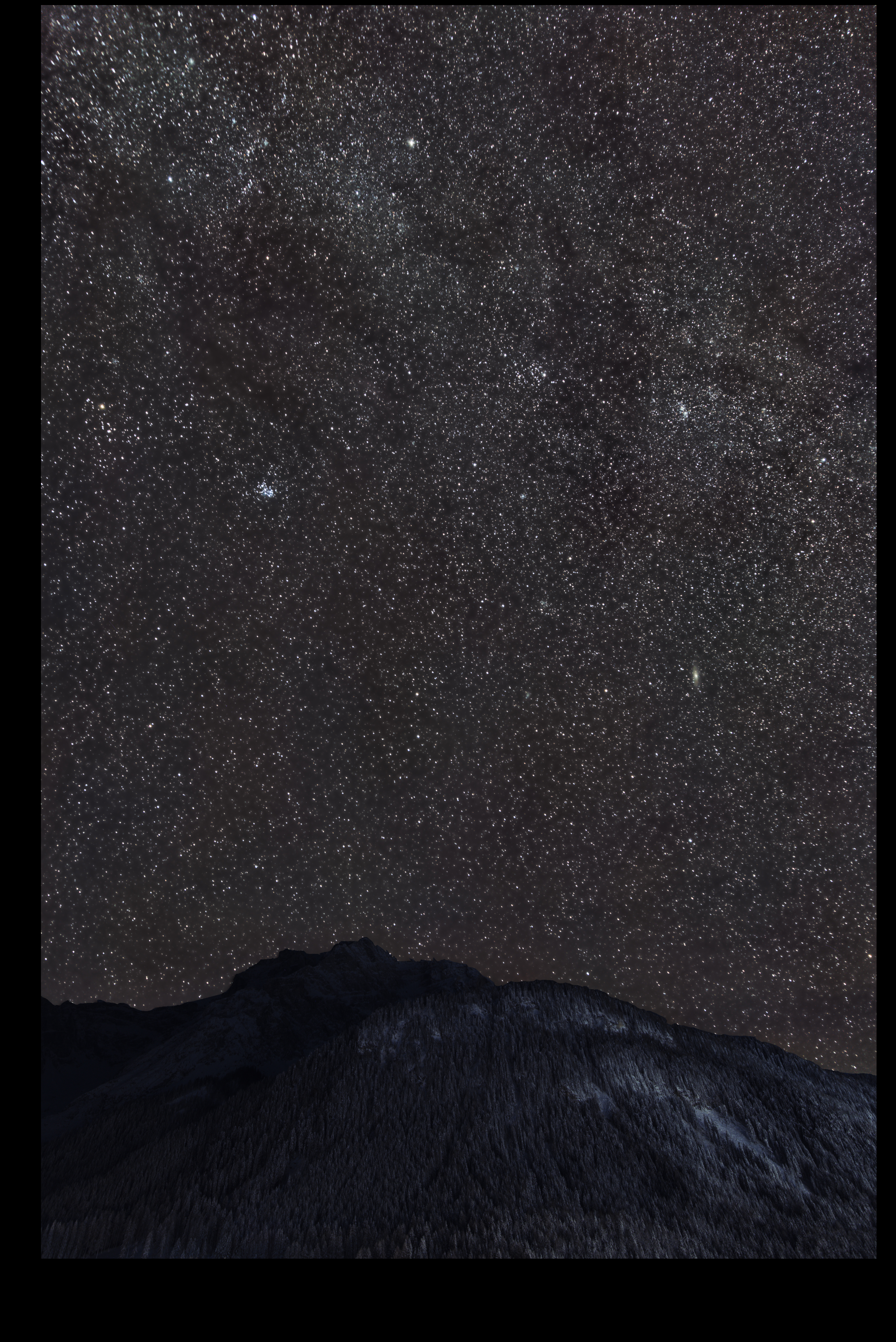
This is the report of my first hands-on to Pixinsight, for which I obtained a trial license recently.
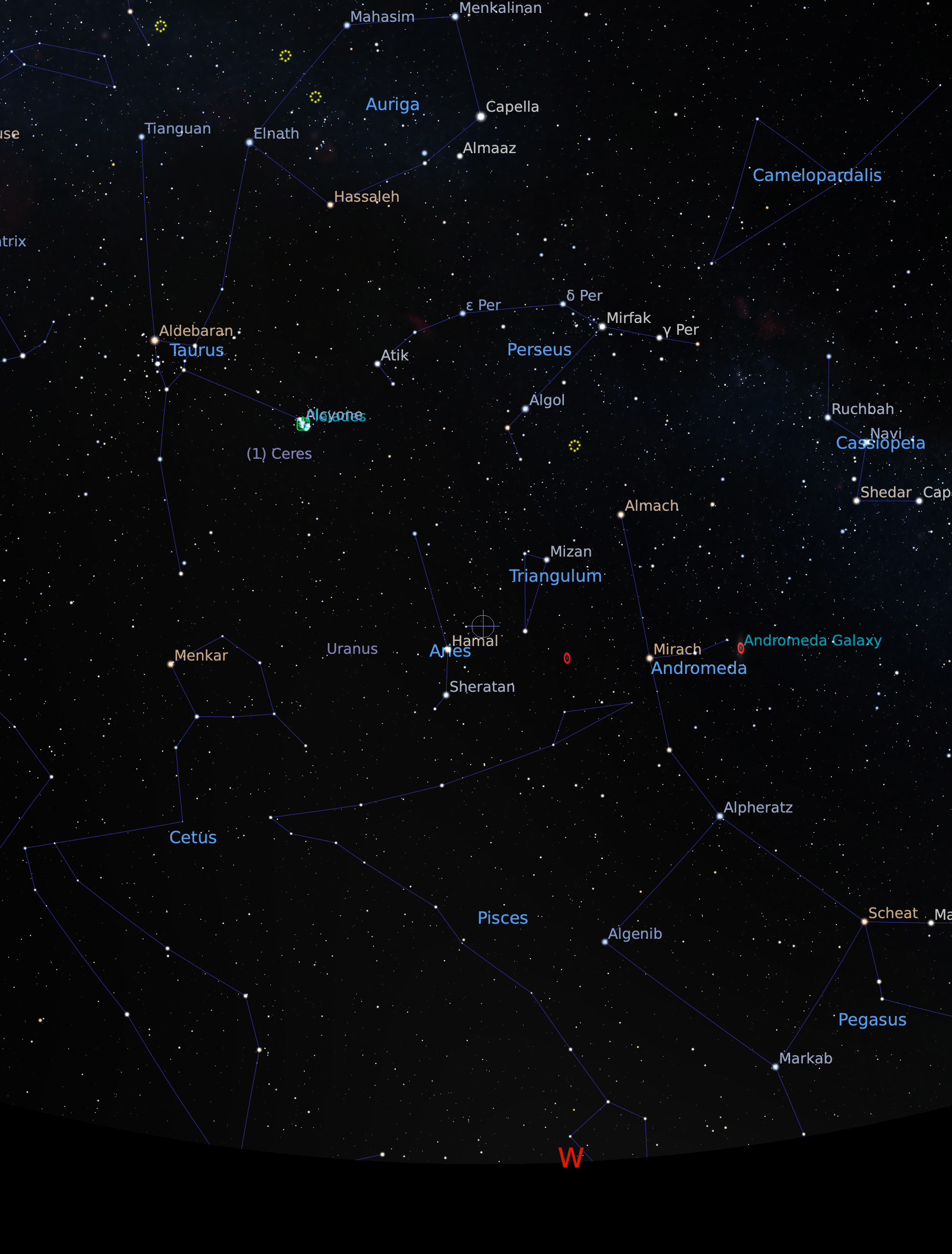
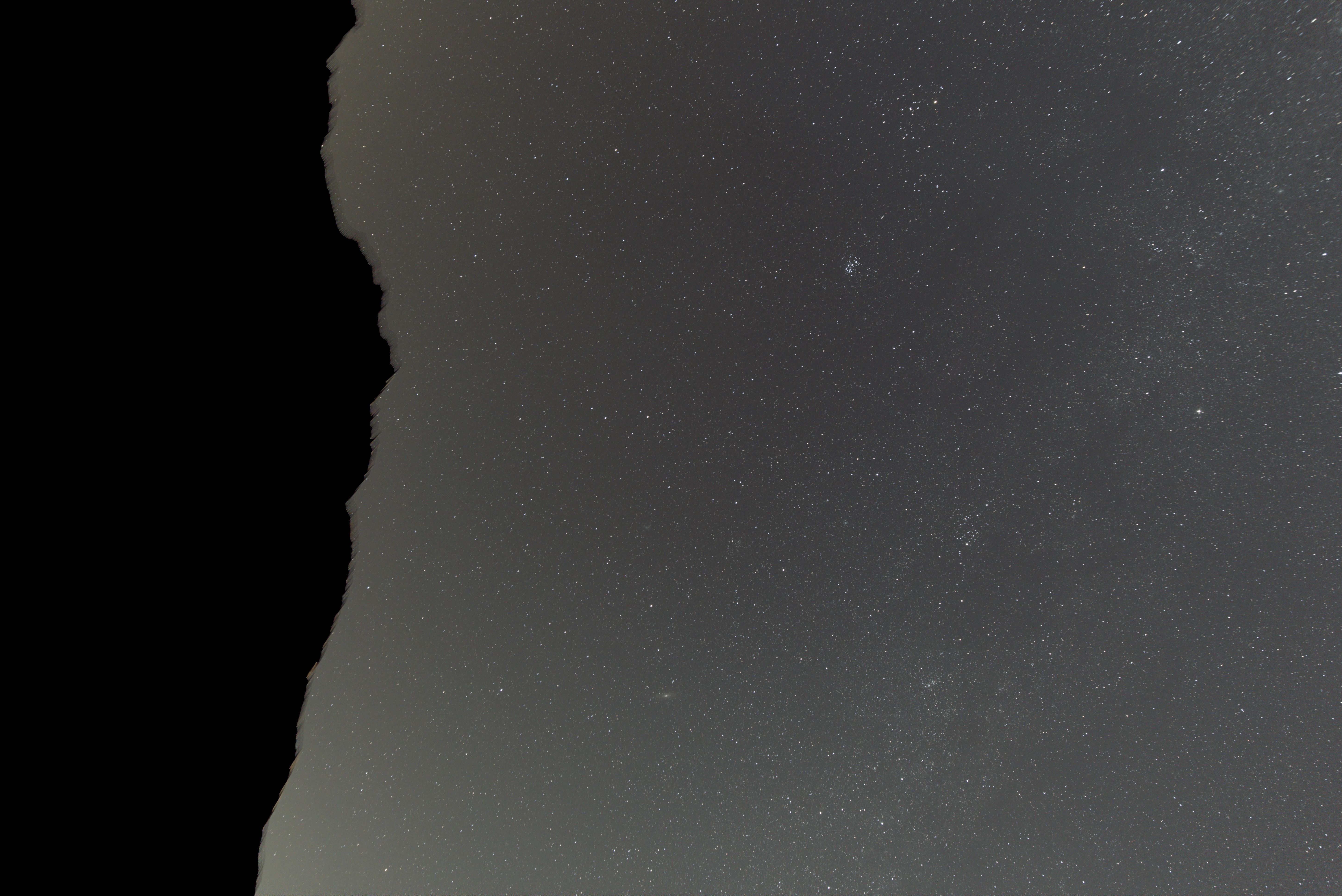
Time, location and target (center of image):
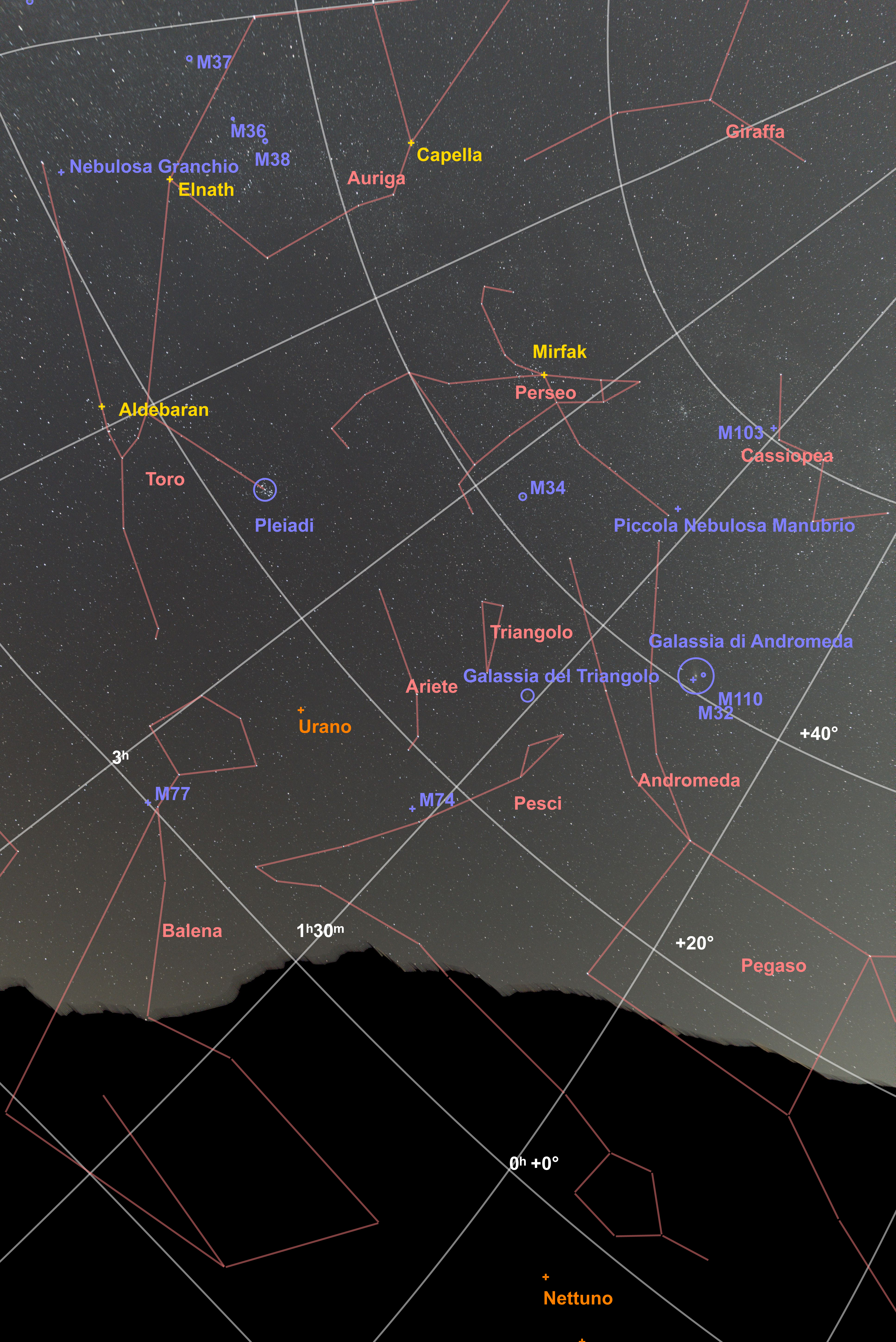
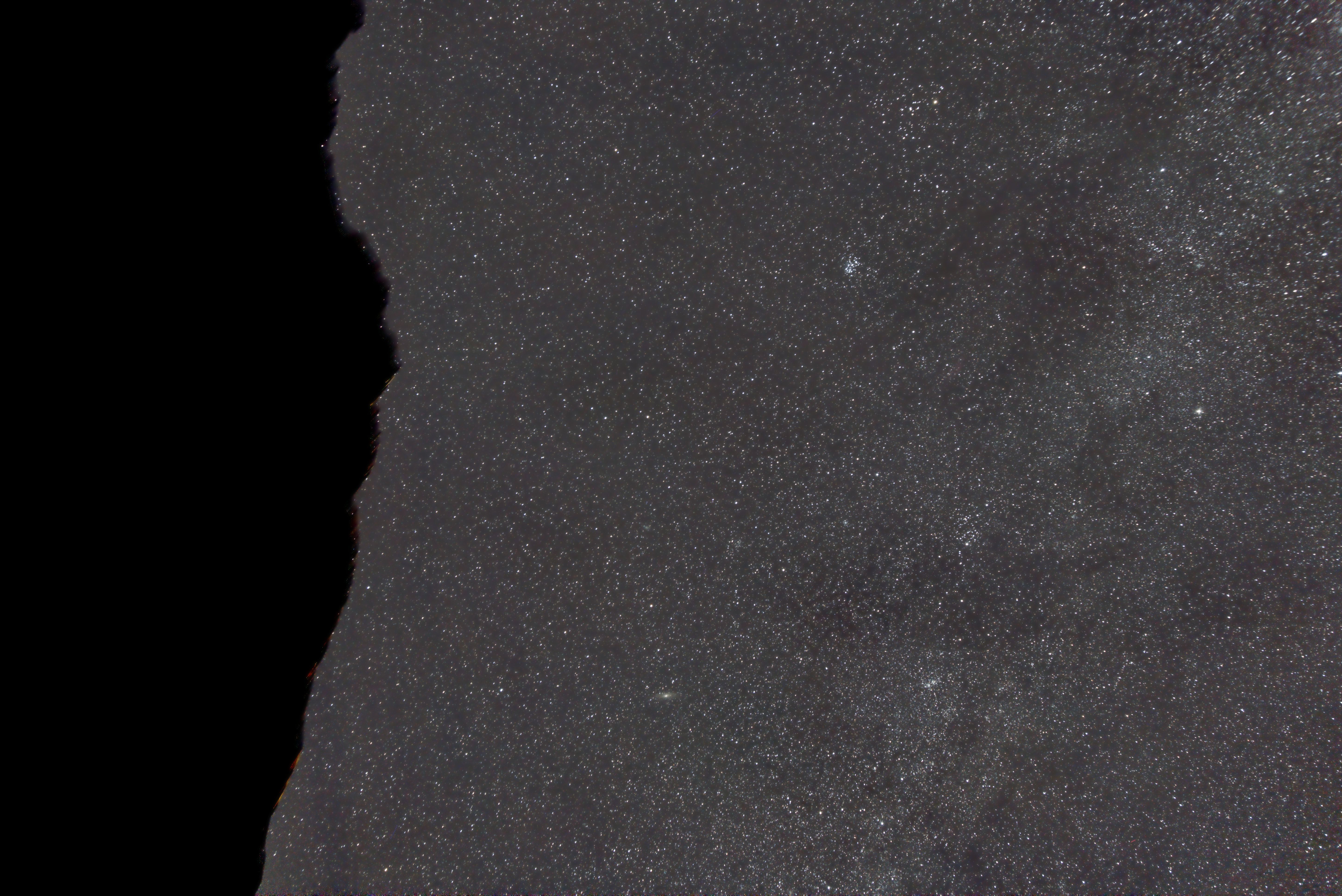
The following image shows the target sky area as depicted by Stellarium.
Equipment:
Camera settings (light and dark frames):
Exposures taken:
Below I will report the result of each of the steps I took in the post-processing workflow (mainly as adviced here).
For each step, I will report
Let's beging with calibration and integration.
|
Let's start with the master bias frame. This is the result of the integration process of the 60 bias frames: |
||
|
|
|
|
Of course the original linear data was heavily stretched here merely for display purposes. Linear signal data is ( 3.128 ± 0.016 ) e-2 on a normalized [0,1] scale. |
||
|
Now let's have a look at the master dark frame, resulting from the integration of the 10 dark frames: |
||
|
|
|
|
Linear signal data is ( 3.126 ± 0.019 ) e-2. A slightly higher value for standard deviation is expected with respect to bias frame, as we are capturing dark current noise and hot pixels here. However, I was a bit puzzled by the lower average value, even though most likely it is not statistically meaningful. I expected a higher average value as I presumed that hot pixels and dark current would mean higher values overall. I also see some evident vertical banding which was not present in the bias frame. This must be the footprint of dark current I guess. |
||
|
Indeed, horizontal and vertical banding appears even more evident by substracting bias from dark (and stretching a lot the result of course): |
||
|
|
|
|
Next, the master flat frame, resulting from the integration of the calibrated (using flat darks, in turn integrated) flat frames: |
||

|

|
|
|
Vignetting is the clear winner here. As a side note: obtaining correct flat frames proved to be one of the most challenging tasks in the whole process. At this extreme wide angle (almost 110° diagonally), just pointing the camera at the sky (even with clear sky) did not provide a homogeneous result, but also using an LCD display was not good enough, as I would need a light source emitting light homogeneously in a 110° viewing angle. Impossible. I always ended up having over-corrected vignetting. Eventually, when I was about to give up, I found that taping a sheet of translucent acrylic glass on top of the LCD display provided (at least apparently) a good source of homogenous light. |
||
|
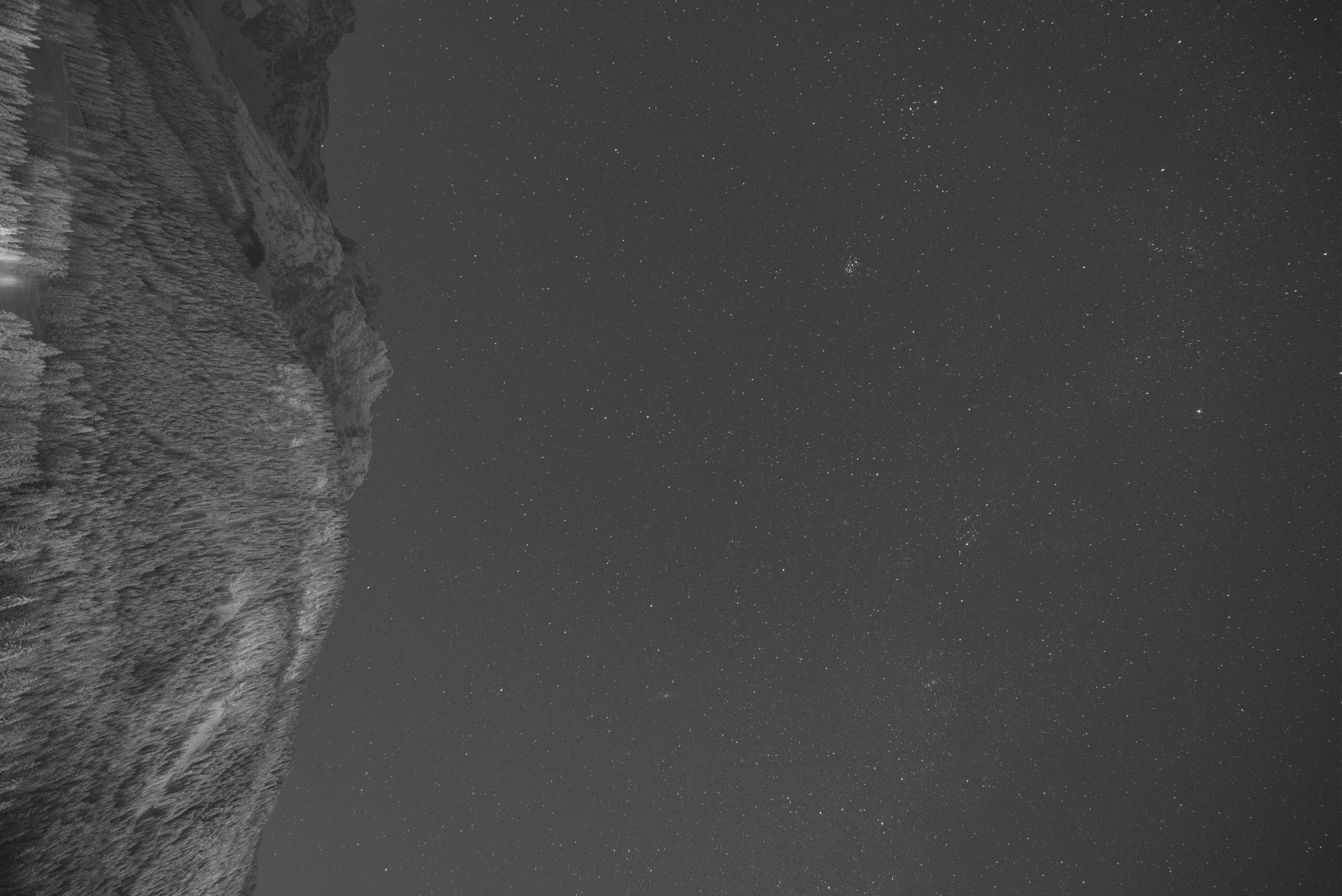
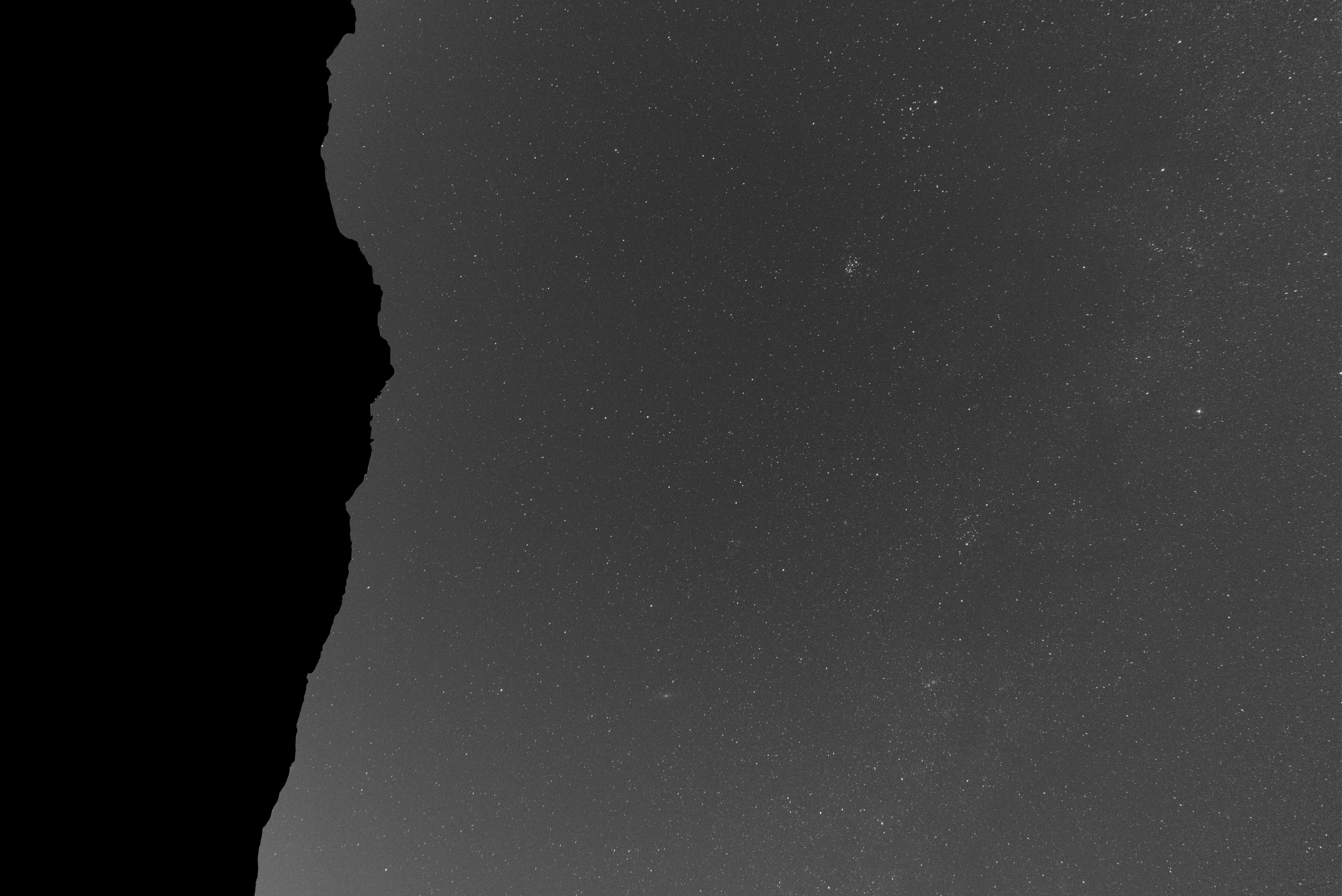
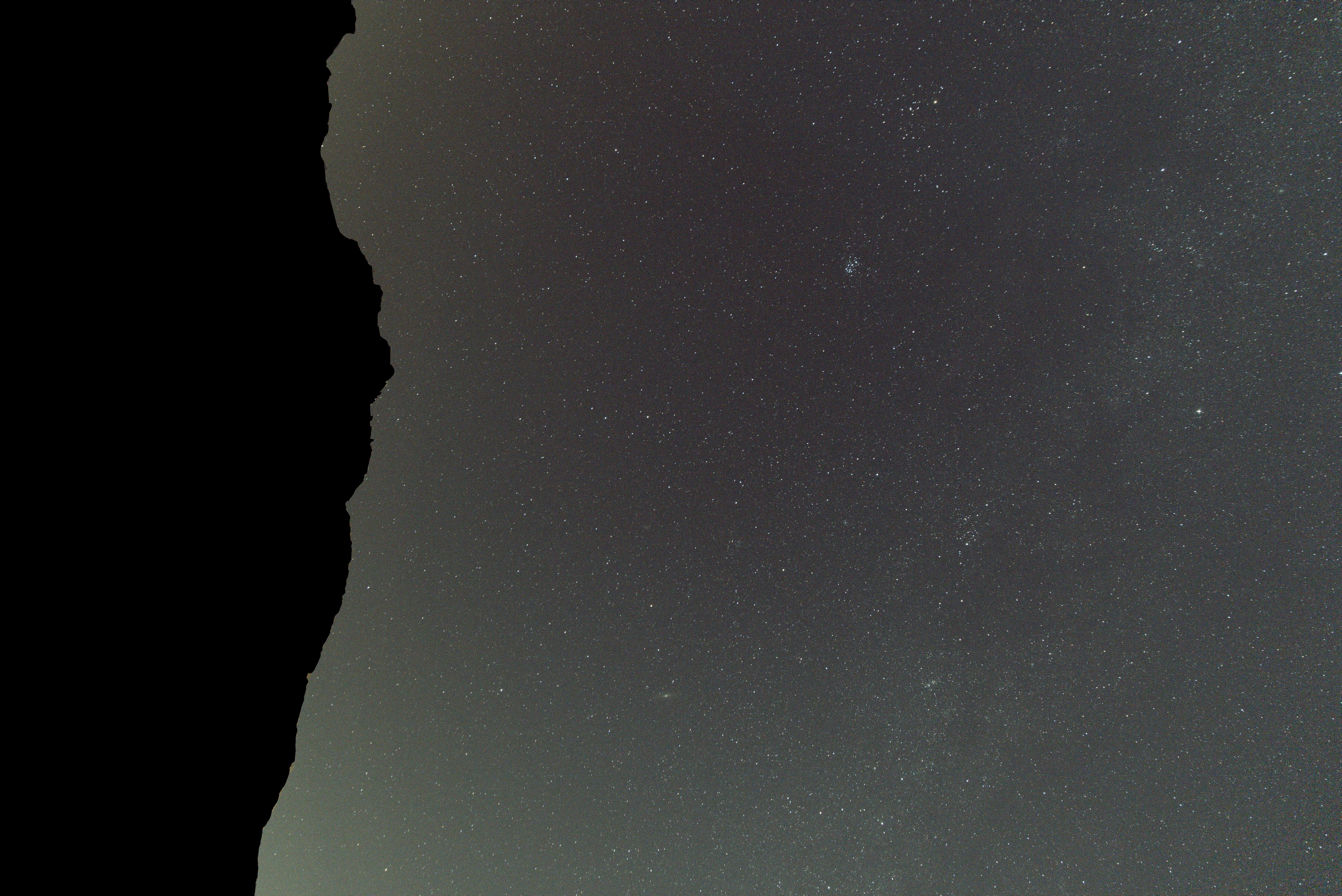
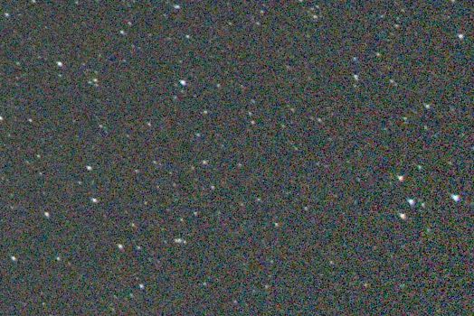
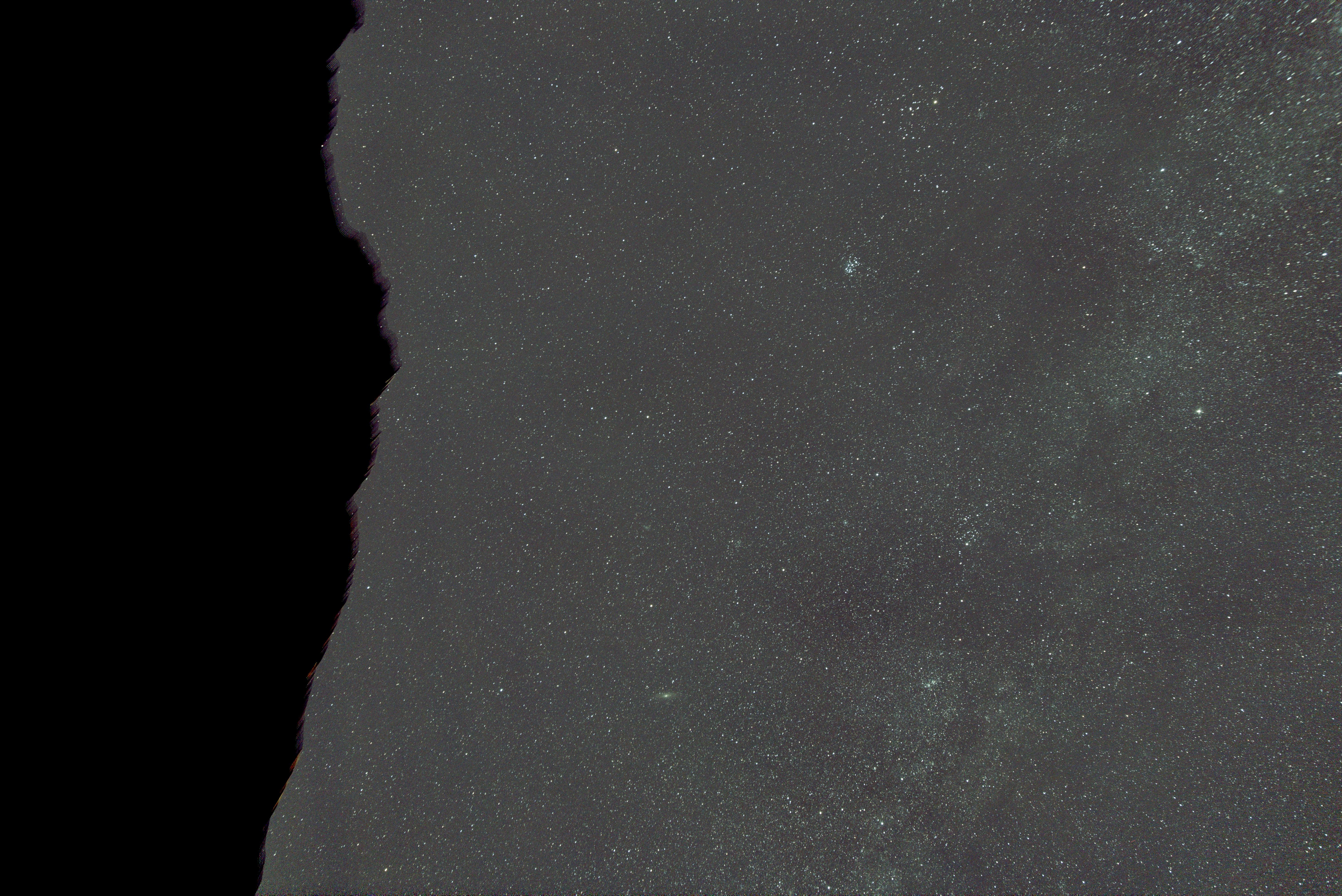
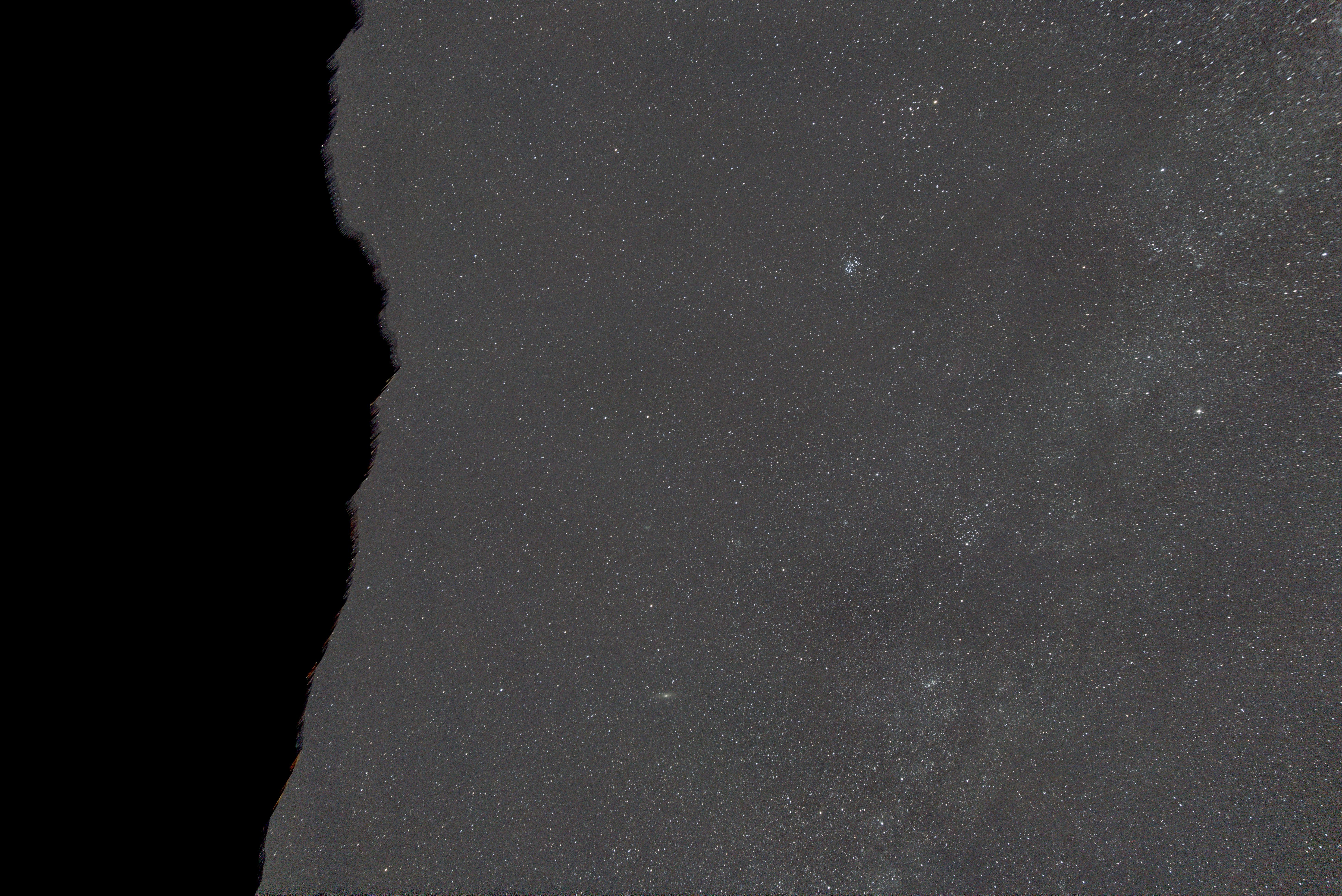
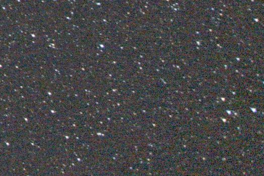
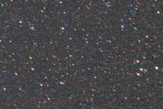
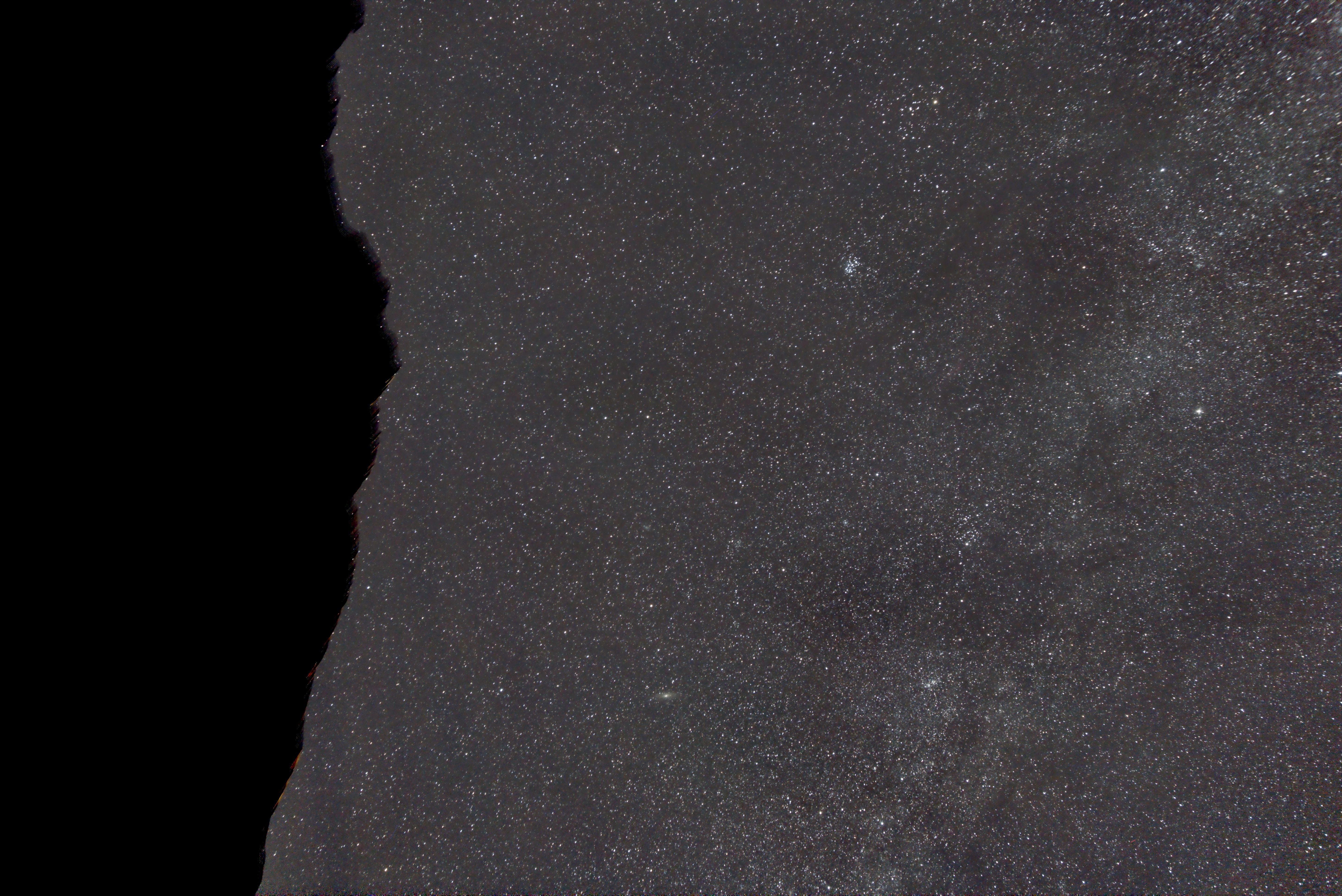
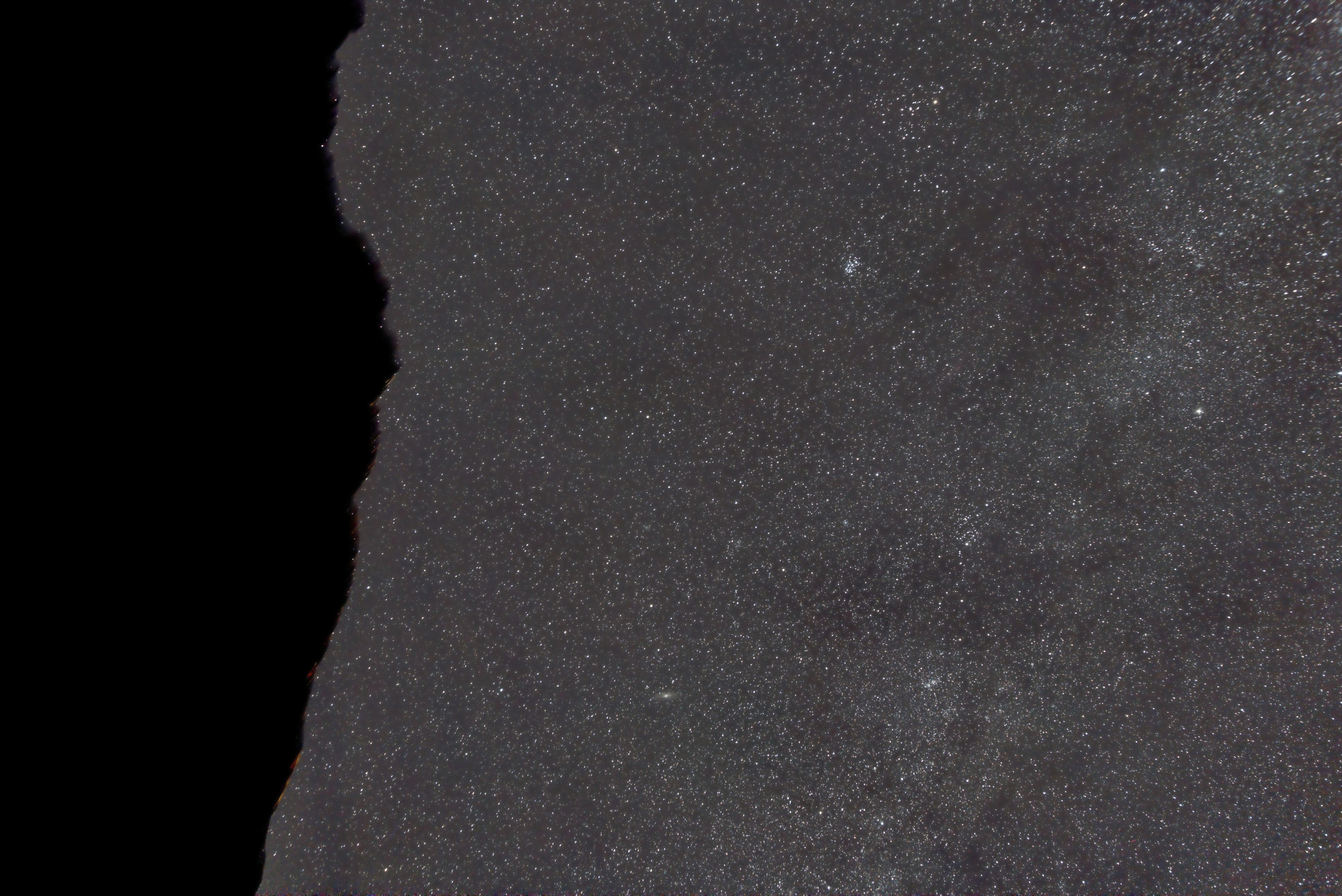
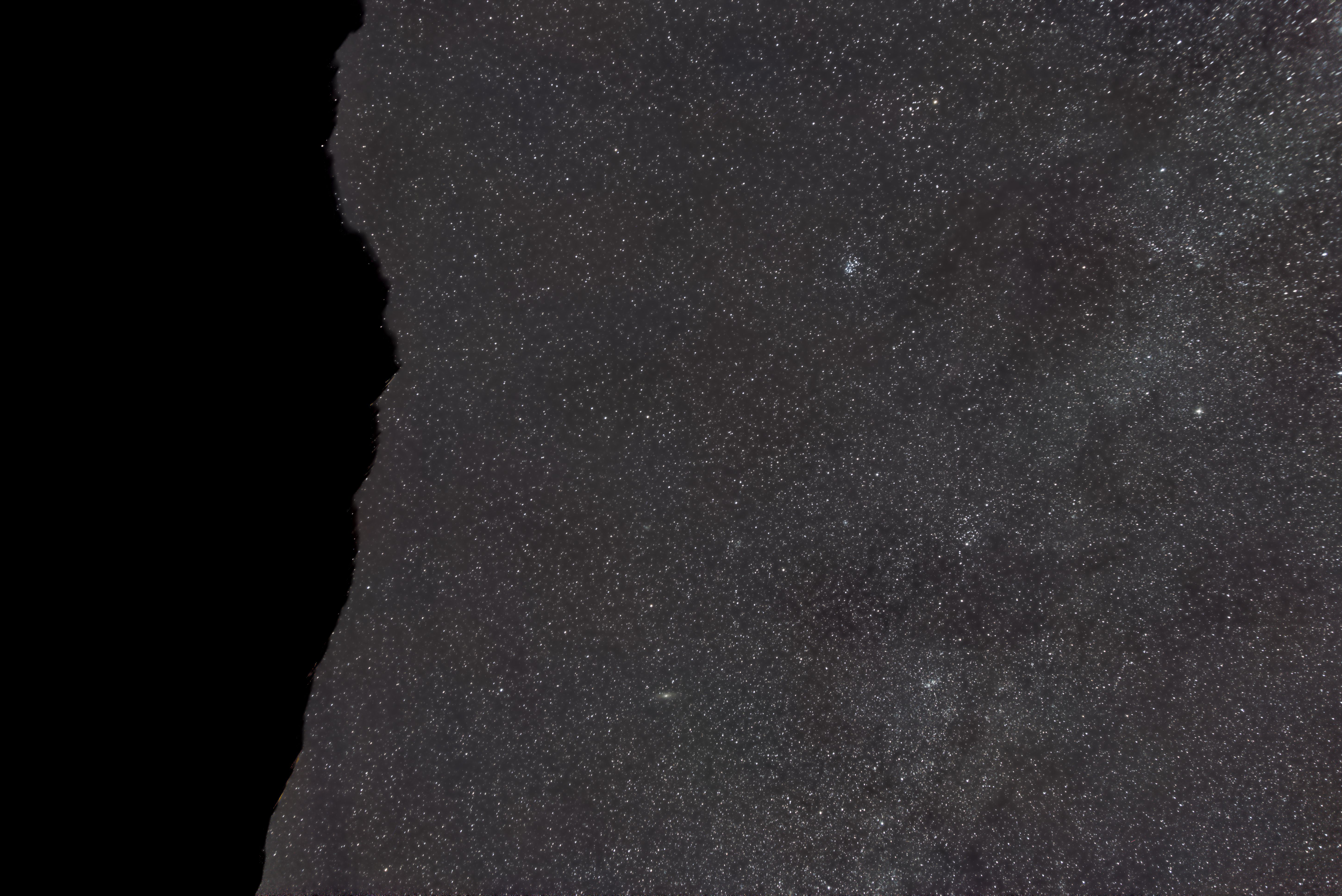
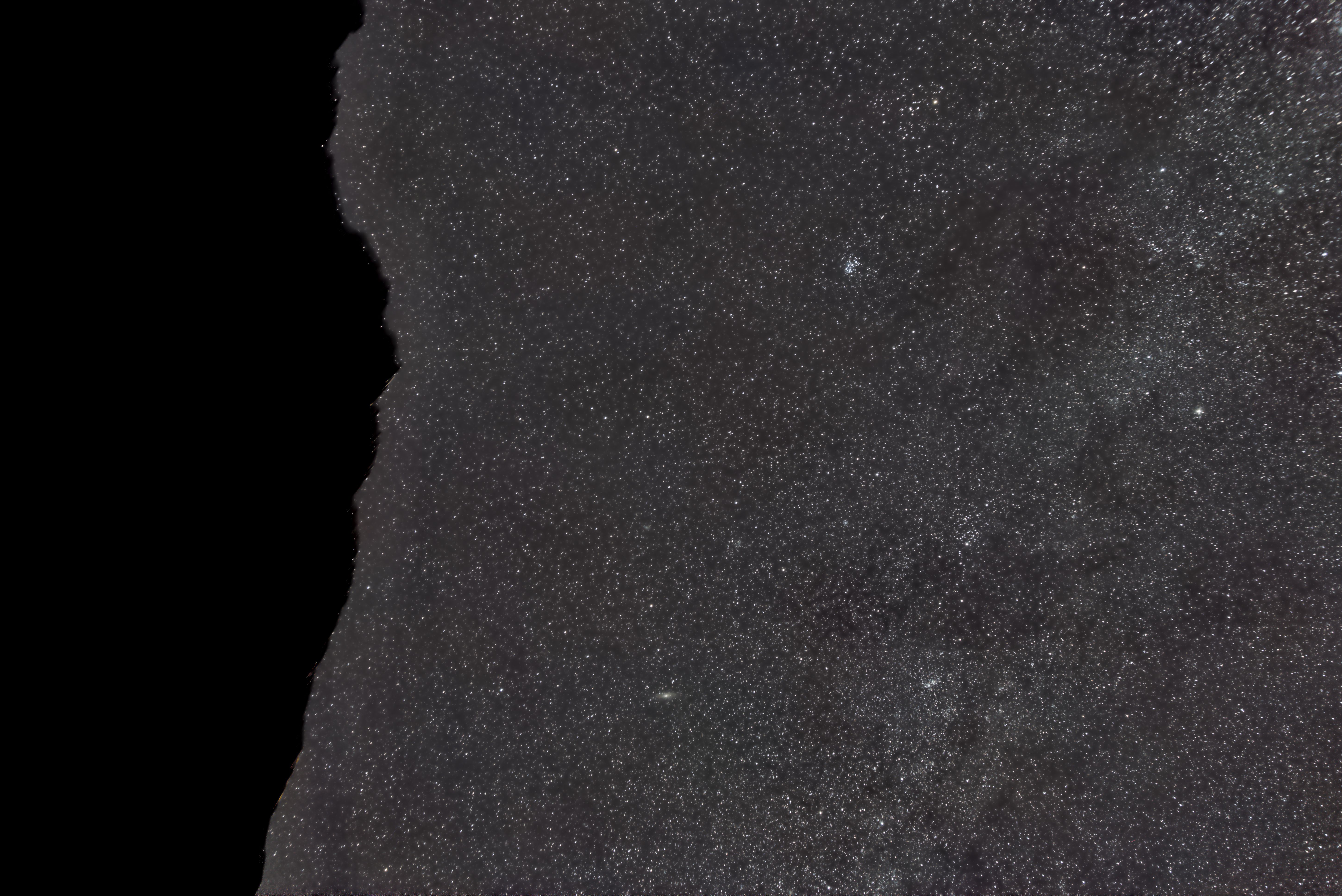
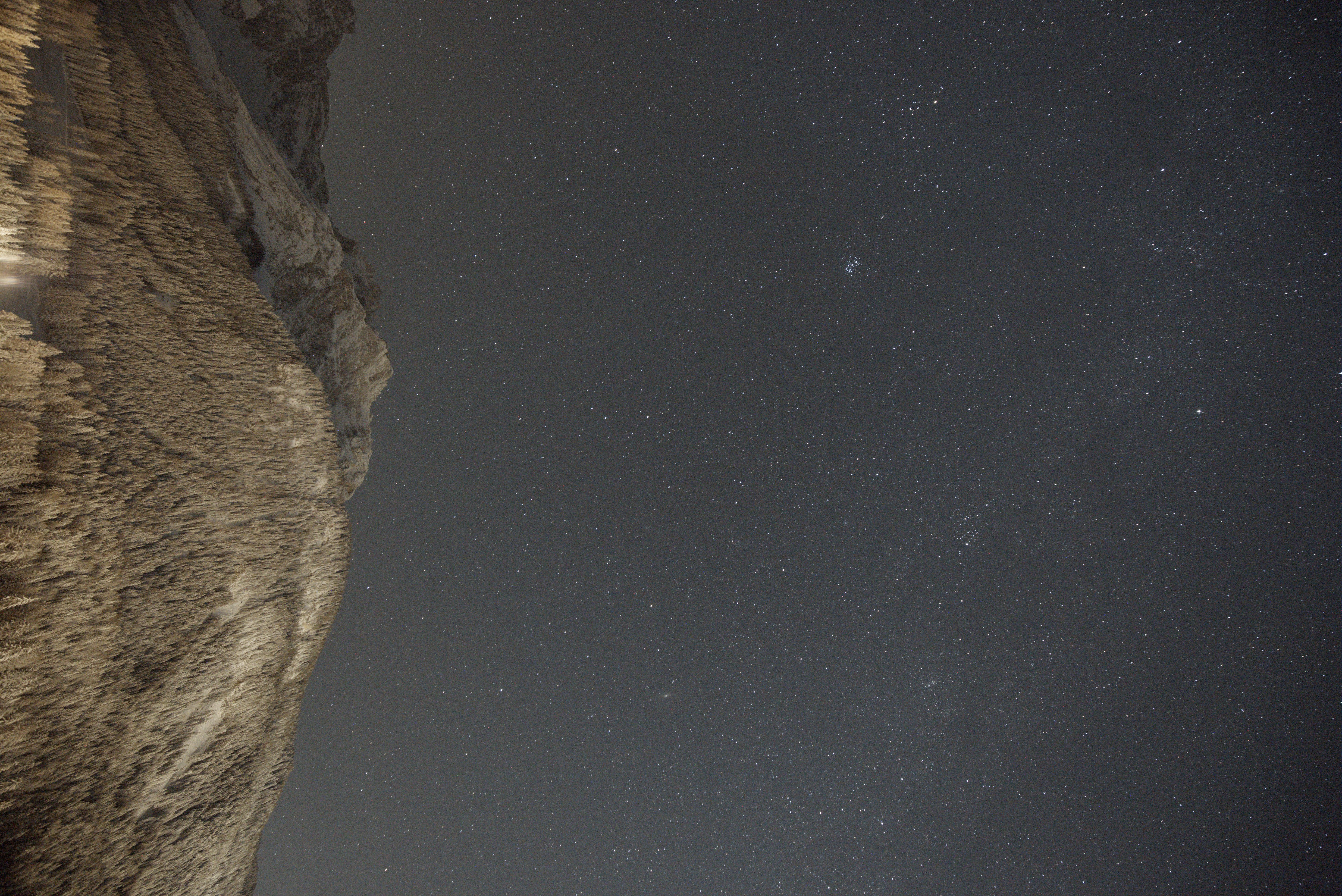
Now, finally, let there be light! So one of the light frames, as an example: |
||
|
|
|
|
Please note that this is not a de-bayered image: to better appreciate this, hover the magnifier over the foreground mountain - you will more easily notice the typical RGGB Bayer mosaic pattern. Just as a reference: linear data has mean ± std dev equal to ( 3.454 ± 0.172 ) e-2. Normalizing this taking as a lower bound my mean bias level @ 3.128 e-2 (seen above) and as an upper bound the level at which my sensor seems to saturate (2.1428 e-1), this translates to 18.9% ± 0.9% of my sensor's dynamic range. Unbelievable how close a "light" frame is to a "dark" one, in terms of average linear value. |
||
|
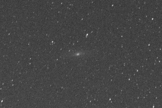
And here the same sample light frame above, but now calibrated using dark, flat and bias masters above (also with foreground subject masked out): |
||
|
|

|
|
It is evident that noise near the corners of the image has worsened, as vignetting removal meant magnifying both signal and noise in these areas. However, to be honest, I still suspect that my flats may be over-correcting. Difficult to say, anyway, as it is clear that the central area of the image is slightly darker than periphery, but this may be well due to light pollution concentrated on the right side of the image, and milky way on top / left. |
||
|
Same frame as above, with cosmetic correction to get rid of hot pixels that were not cured by calibration: |
||

|
|
|
|
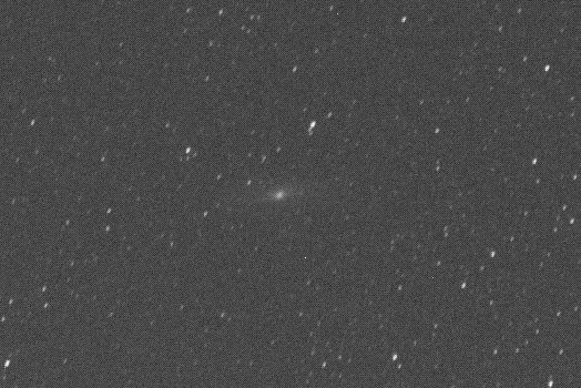
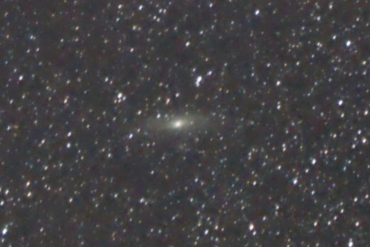
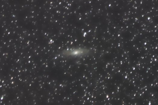
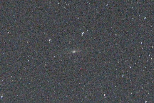
It may be difficult to spot the differences here. However you may find that a hot pixel just on the right of Andromeda's galaxy is gone now. |
||
|
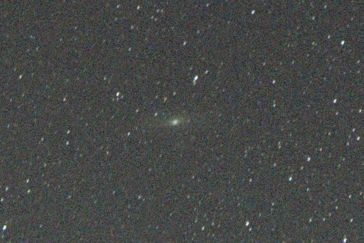
And now let there be color! Same frame as above after de-bayering (or de-mosaicing if you like): |
||
|
|
|
|
The way I understand it, the reason why we are de-bayering before (registering and) integrating, and not after, is that I am not on a tracking mount here, so it would make little sense to integrate single RGGB pixel arrays with a moving target: indeed, even after registering images, the same light source may fall on a Red pixel in one shot, on a Green one in another, and on a Blue one in a third one. |
||
|
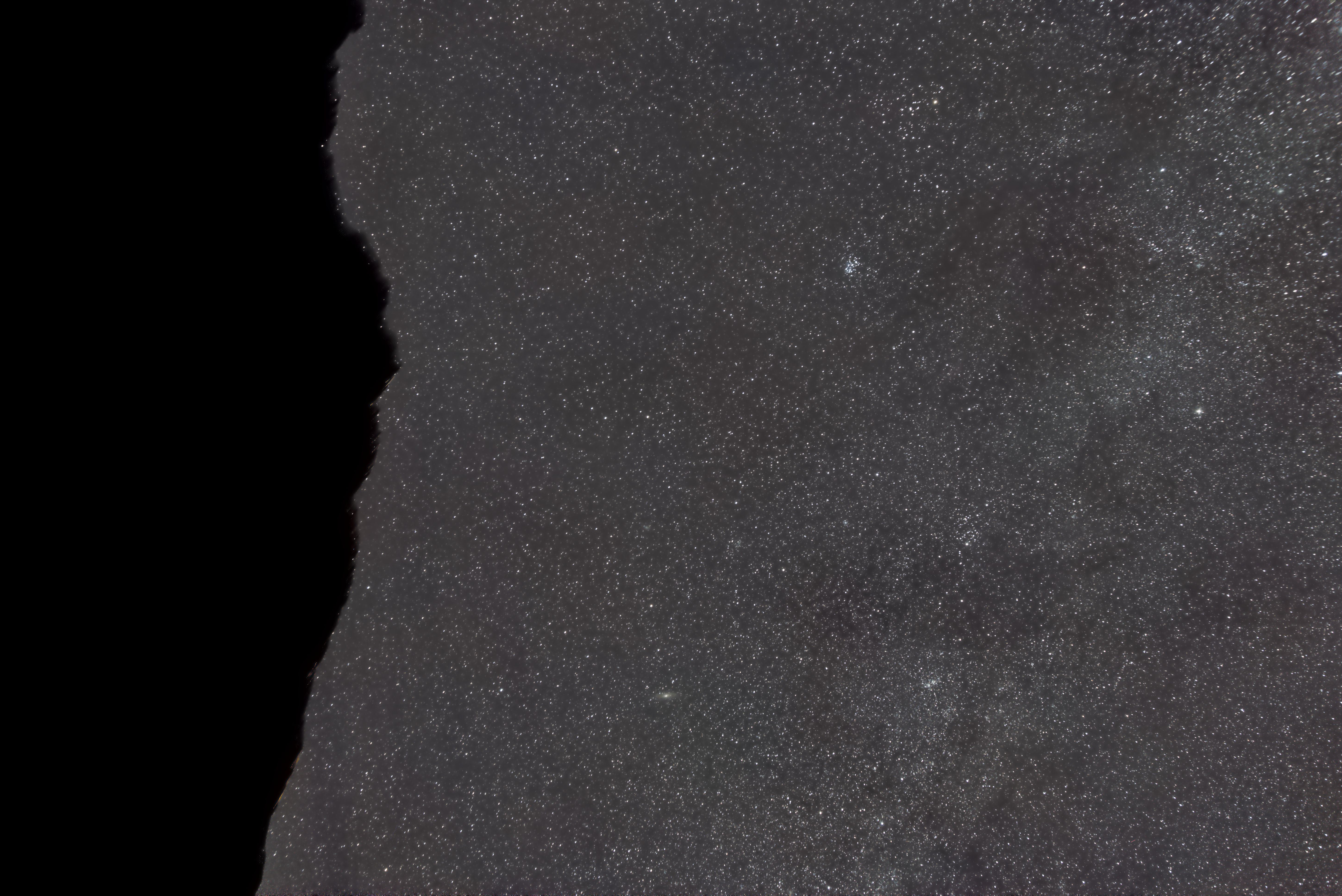
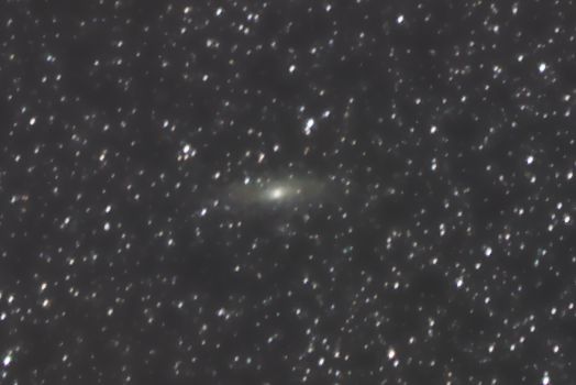
And finally the result of the integration of the 10 frames, after registering: |
||
|
|
|
|
As expected, noise reduction is massive in this step. |
||
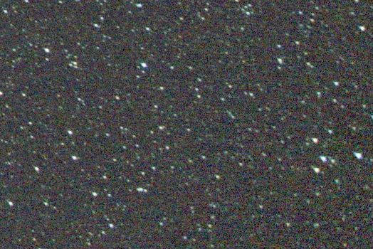
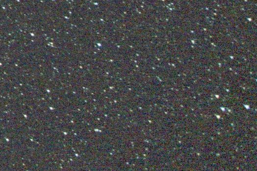
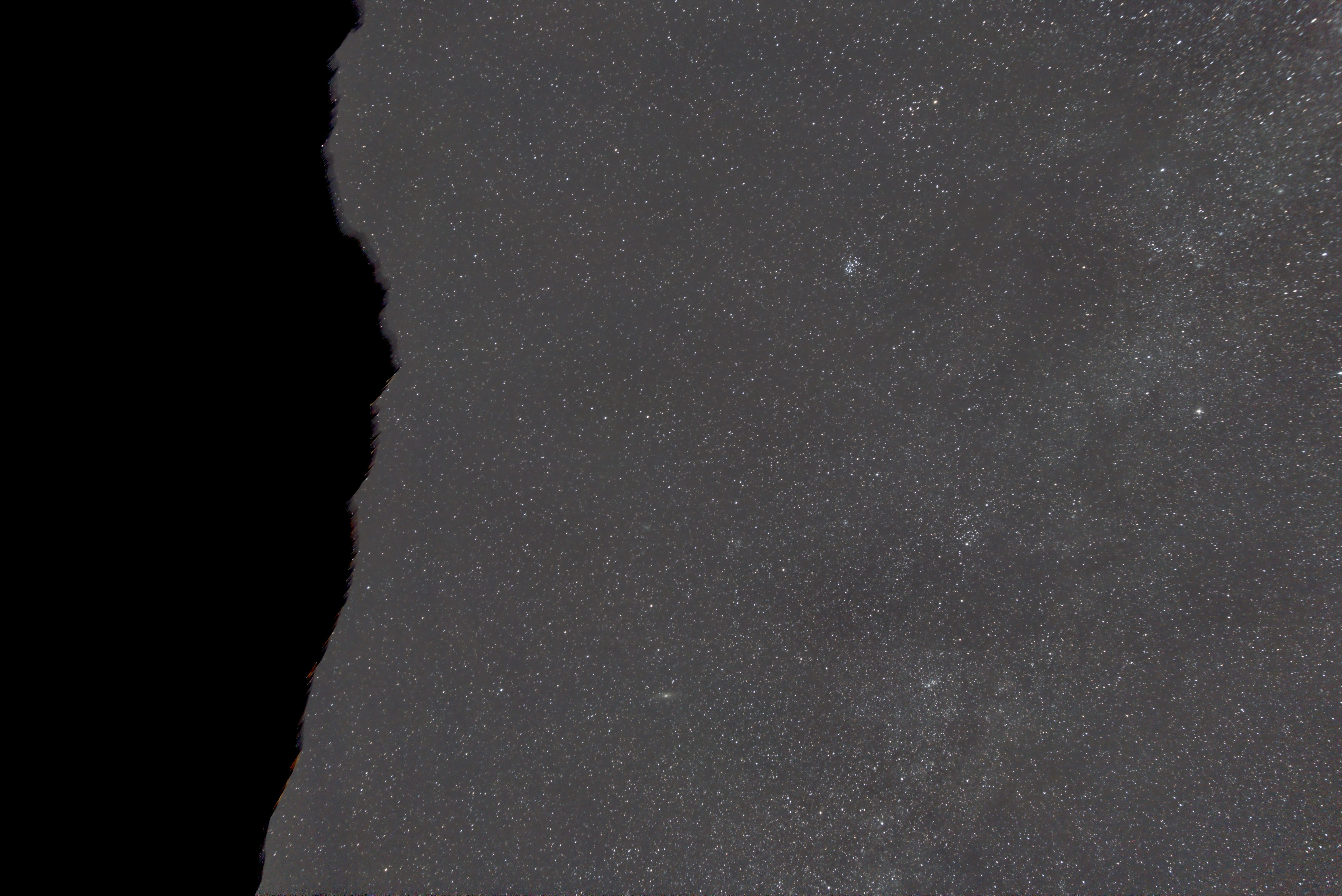
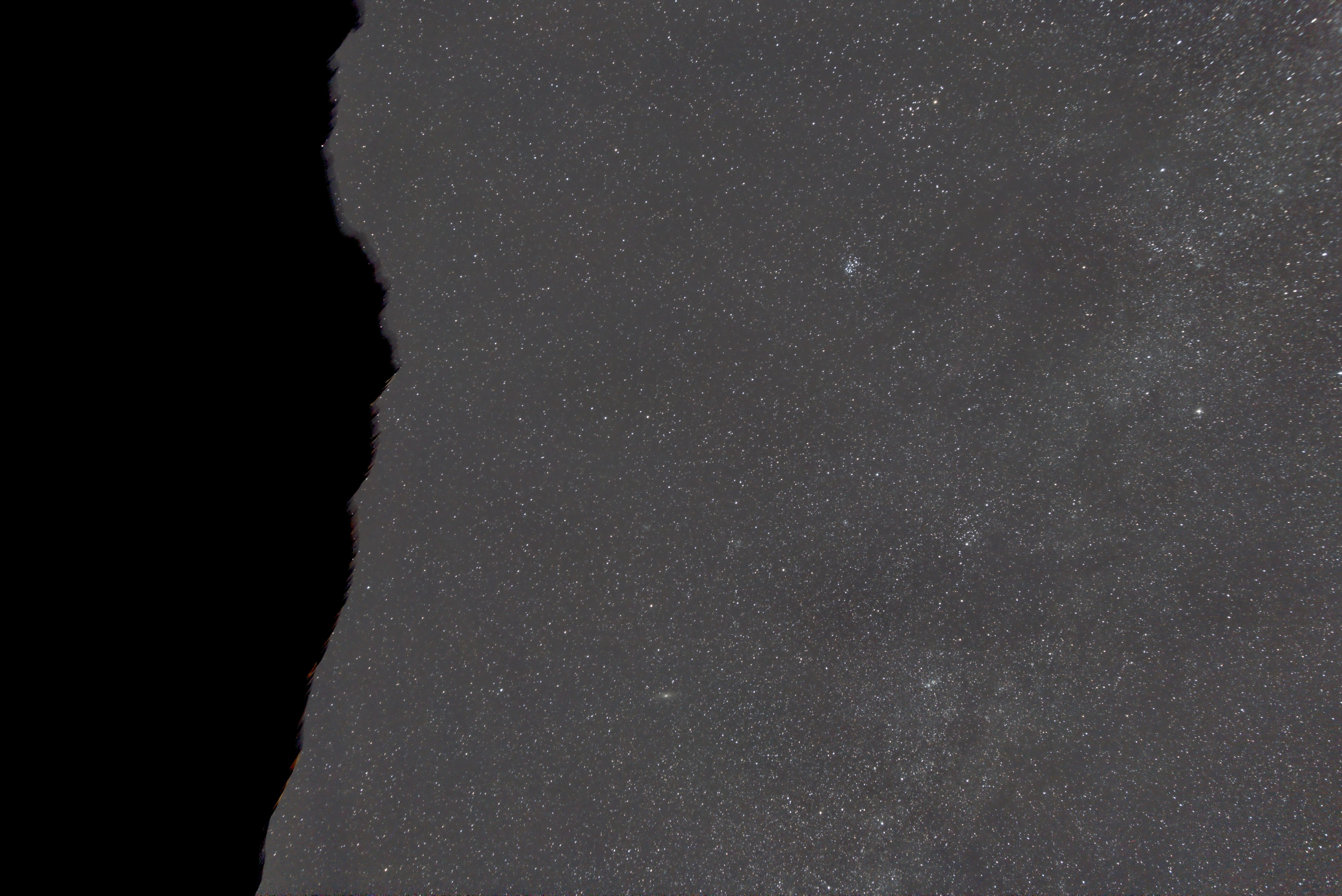
Time to have a look at what we have done so far! On the left, the original sample light frame, here represented as de-bayered and with foreground masked in order to simplify comparison with the right, which is the final master light frame.
|
|
|
|
With a 0.1x zoom, noise reduction is not particularly noticeable. What is evident is the de-vignetting achieved thanks to flat frame substraction -- once again, is it over-correcting? Difficult to say, but it may be the case. However, we know that Dynamic Background Extraction may later fix this somehow. |
||
|
|
|
|
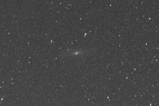
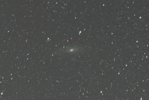
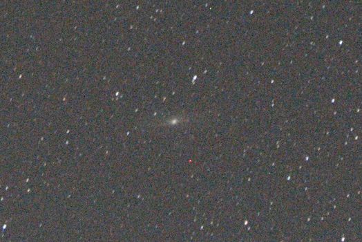
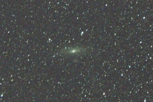
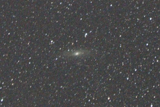
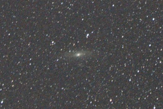
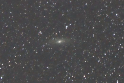
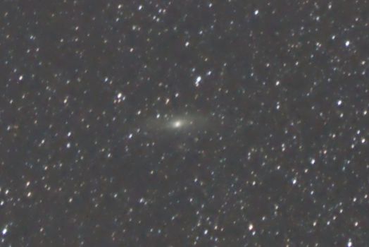
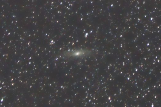
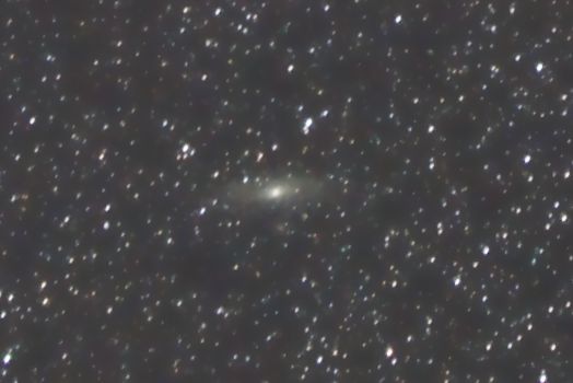
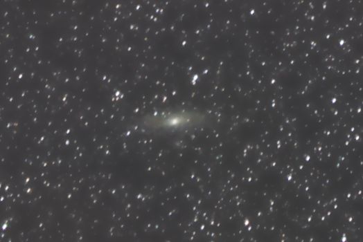
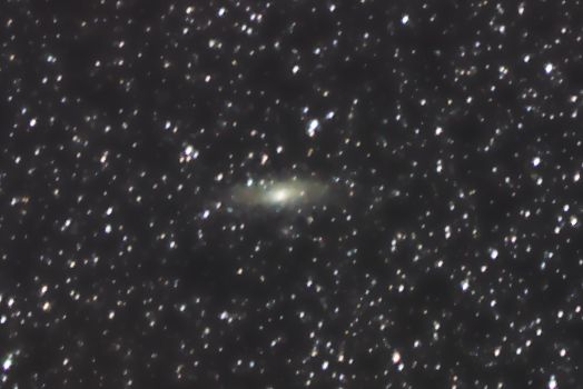
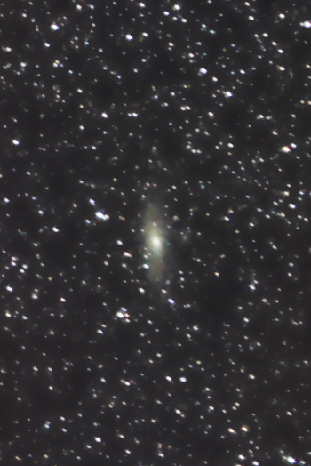
Andromeda galaxy has definitely gained from the calibration and integration process -- its disc now clearly stemming from the background. Also, the removal of the red hot pixel is more evident after de-bayering. |
||
|
|
|
|
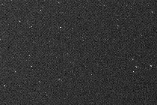
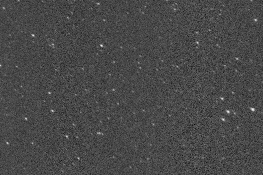
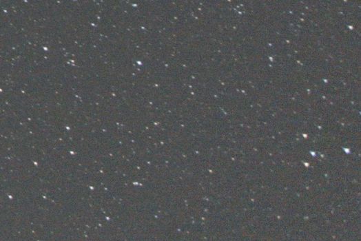
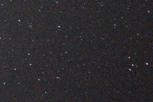
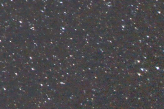
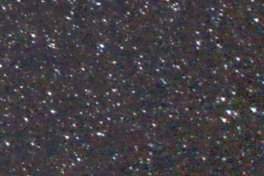
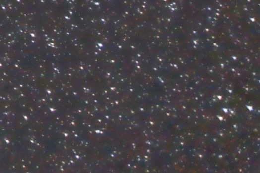
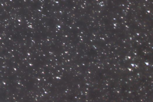
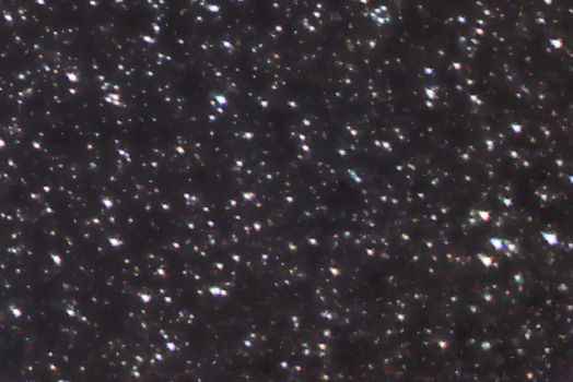
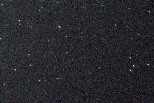
The outer area near the top-right corner has undergone massive amplification to correct for vignetting during the calibration phase, and noise reduction achieved through integration is very clear. Also in this case a hot blue pixel has been removed thanks to Cosmetic Correction. |
||
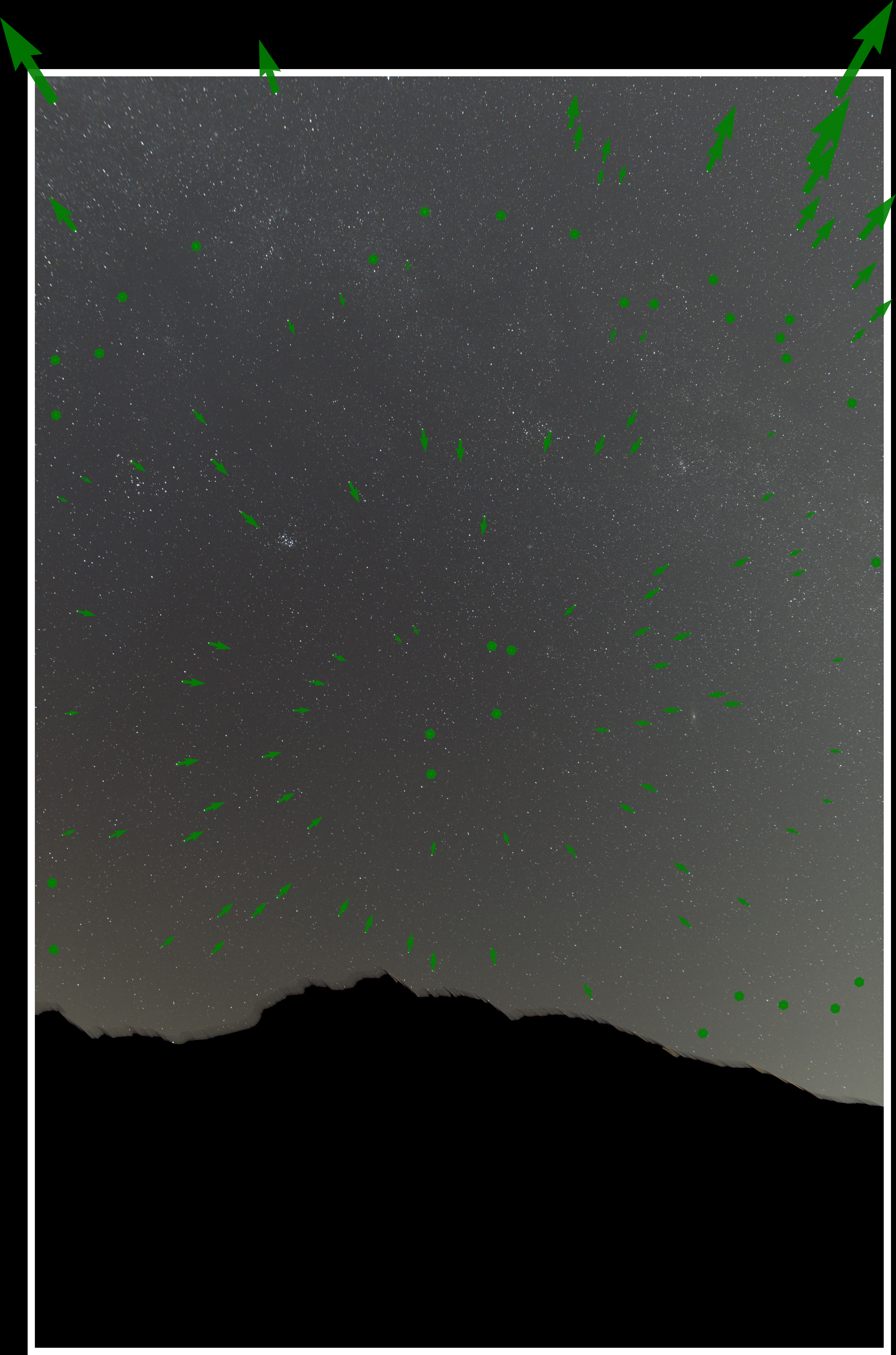
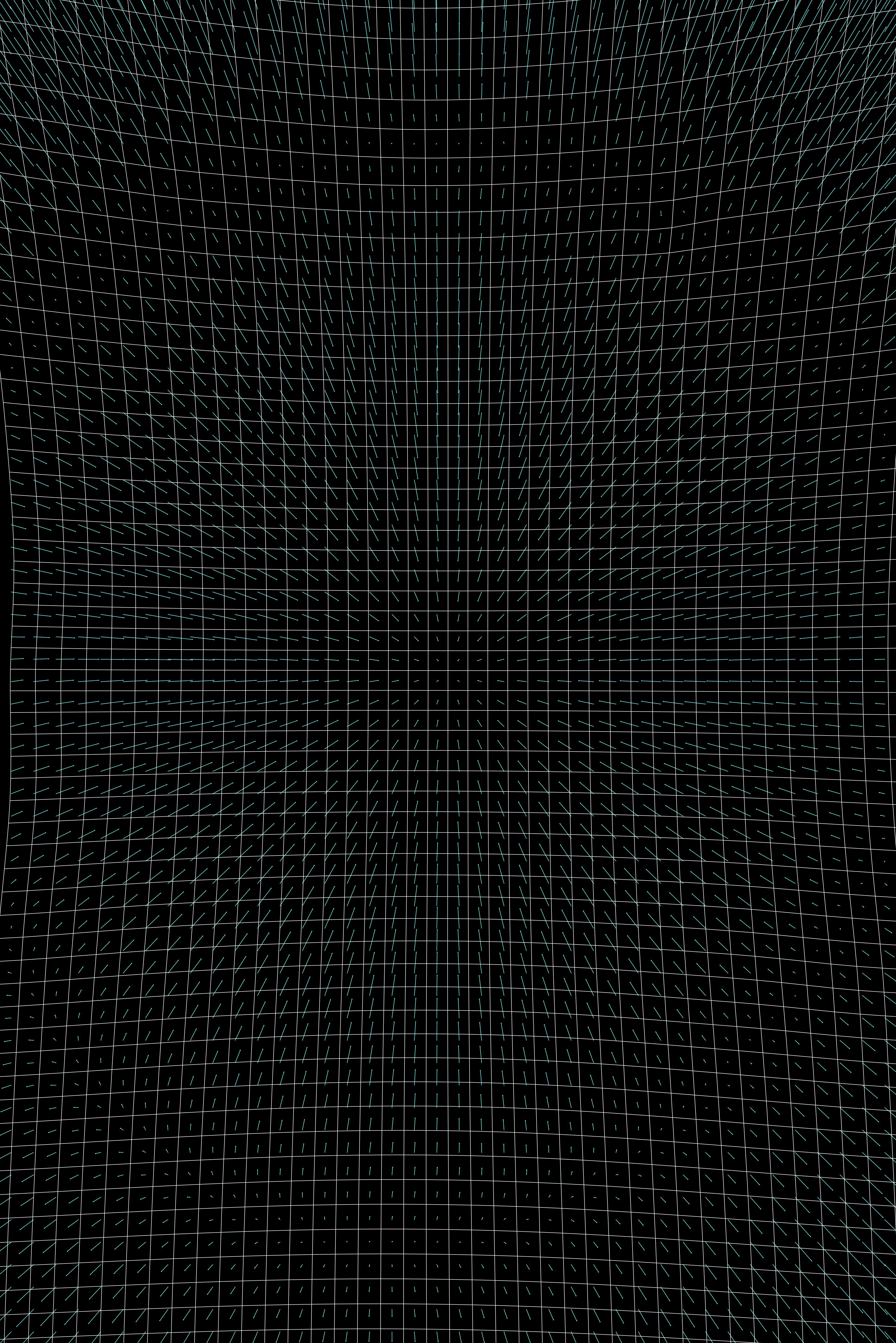
Since I wanted to try color calibration via the magical Photometric Color Calibration tool, I needed to plate-solve my image. This proved to be pretty hard, given my lens strong distortion, so that Image Solver could not succeed. In the end, I had to follow the steps below:
The following couple of images displays
×
|
×
|
By the way, the green vector field I represented on the left image is just a depiction of the .csv file representing the distortion model as produced by Manual Image Solver (rendered in Python and overlaid on the master light frame)
Finally, here comes the plate-solved light master (sorry for the Italian!):
Now we are ready to tackle color balancing.
|
So let us start from where we finished, namely the light master frame: |
||
|
|
|
|
|
The first step is maybe the most dramatic one, i.e. the removal of light pollution-induced gradient via Dynamic Background Extraction: |
||
|
|
|
|
Pretty striking. Having removed a yellow cast, the image now has a green cast left over. That will be addressed by the color balancing procedure. |
||
|
Now, I tried neutralizing background via Background Neutralization: |
||

|

|
|
|
To be honest, I am not impressed by this step. It seems to leave things unchanged at the best. Not sure if I'm doing something wrong here. |
||
|
Now, a long-awaited step, namely color calibration using Photometric Color Calibration (which required plate solving, see previous section): |
||
|
|
|
Next figure shows the PixInsight Photometric Color Calibration tool final report.
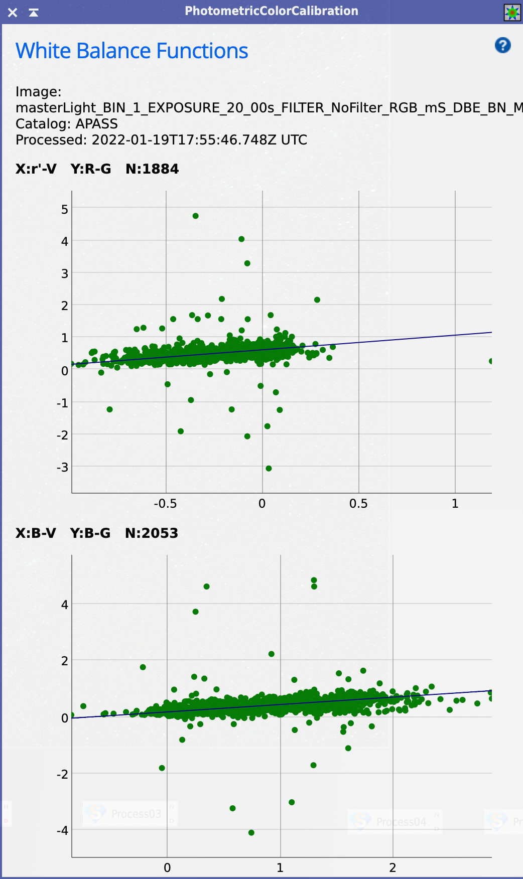
There seems to be some big dispersion here, which may point to a not-so-accurate color balancing, though y scale magnitudes of the scatter plots do not help in assessing this.
|
Next, from my understanding, assuming that color balancing is now correct I should not see any green in our sky, so green-ish pixels left should only be the consequence of noise. So this is the time to try and fix this by Subtractive Chromatic Noise Reduction: |
||
|
|
|
|
I had to use this tool with great caution to avoid the emergence of a red cast in particular near the corners of the image. I think that I should have been more aggressive overall with this, if that did not cause problems near the corners. |
||
|
And now to noise reduction. First pass using Multiscale Linear Transform on small-scale RGB/K components: |
||
|
|

|
|
The effect is evident. Of course noise reduction was applied more aggressively to dark areas, thanks to a mask that was built simply starting from the stretched version of the (linear) image (stretched as suggested by automatic settings of Screen Transfer Function). |
||
|
With the same mask on, I took a second noise reduction step with Multiscale Median Transform, once again on small-scale RGB/K components: |
||
|
|
|
|
Not particularly impressed to be honest. |
||
|
Time to stretch the image! Images shown so far were still in a linear state, and were stretched only for display. Check result below of Histogram Transformation, set to my personal taste: |
||
|
|
|
|
Having stretched a bit more than suggested by automatic Screen Transfer Function settings, in order to make contrast pop out a bit more, some 'dark bubble' pattern emerges in the background, and noise kicks back in particularly near the corners. |
||
|
So let's have another pass with Multiscale Linear Transform: |
||
|
|
|
|
Once again, noise reduction was performed more aggressively in dark areas, this time taking as a mask the very same image luminance (extracted by Channel Extraction in the CIE L*a*b* mode). |
||
|
With the same mask on, let's take a pass with ACD Noise Reduction: |
||
|
|
|
|
A great enhancement particularly near the corners. |
||
|
Now we want to get rid of the chromatic noise spread all over the background, once again with Multiscale Linear Transform, this time with large-scale Chrominance (instead of small-scale RGB/K components) as the target: |
||
|
|
|
|
The result is impressive, particularly near the corners. In order to avoid attacking and harming in any way stars and deep sky objects with this aggressive chrominance noise reduction, a mask was used using Range Selection, in order to obtain a more binary 0/1 mask. |
||
|
We are in a position now where we may afford a further slight stretch in order to make contrast pop a little bit more, so let's do it: |
||
|
|
|
|
Did I push too far? Maybe. Noise looks low to me, but some dark blotches have been emphasized. However, I decided to live with it as I like the overall effect of this second stretch. |
||
|
Finally, some slight contrast increase in strong signal areas. Of course this is not particularly important with this kind of subject, lacking a prominent DSO object. However, I wanted to take practice in this procedure. So here it is, a slight touch of local contrast via Local Histogram Equalization: |
||
|
|
|
|
In order to attack only strong signal areas, a mask was built as the union (addition) of two masks, that were generated separately via Star Mask and Range Selection. I also took the chance to enhance slightly contrast on the negative mask, though I'm not 100% sure it was a good idea after all. As a side note, for some reason beyond my comprehension, this process yields a sort of brighter halo on the horizon -- which I will later correct in PhotoShop. |
||
|
Final step! Slight contrast and saturation boost using Curves Transformation: |
||
|
|
|
For the foreground, I just integrated the calibrated light frames without registering them. Then I stretched the image and adjusted it (mainly for color balance) to taste.
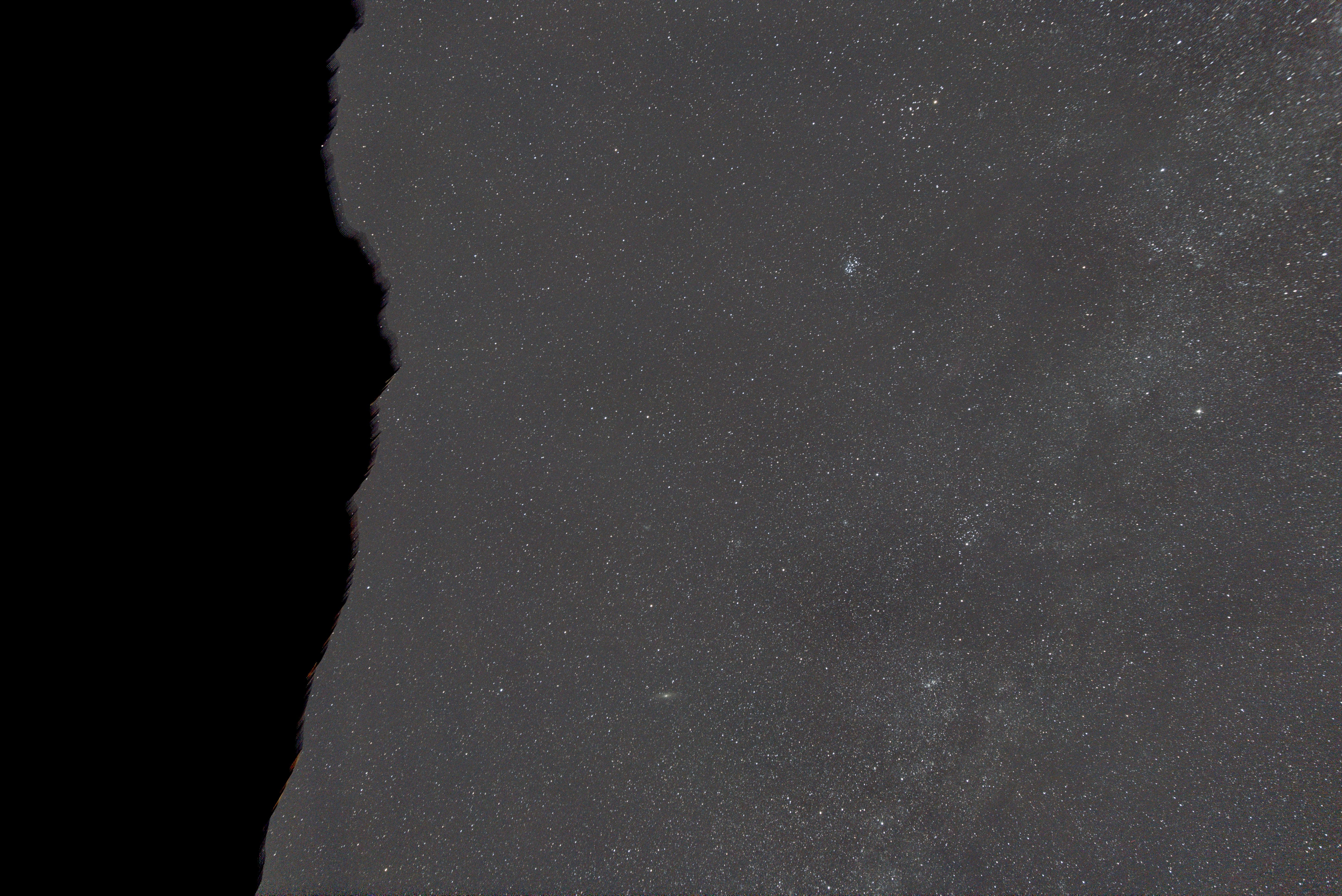
So this is it! On the left, the original sample light frame, here represented as de-bayered in order to simplify comparison with the right, which is the final image. Please note that I had to crop the final image a bit.
|
|
|
|
|
|
Thank you for reading!